ML Intensive for TLF
Lecture 4. Linear models, Stochastic Gradient Descent
Alex Avdiushenko
August 20, 2026
In the last episode
- ML types: Supervised, Unsupervised, and Reinforcement Learning
- Linear Regression model
- Train/Test splitting and overfitting
- Significant events in ML
Training Regression as Optimization Task
Training sample: $X^\ell = (x_i, y_i)^\ell_{i=1}$, $x_i \in \mathbb{R}^n$, $y_i \in \mathbb{R}$
Linear regression model (weights $w \in \mathbb{R}^n$):
$a(x, w) = \left< w, x\right> = w^T x= \sum\limits_{j=1}^n w_jf_j(x)$
Squared loss function:
$\mathcal{L} (a, y) = (a - y)^2$
Training Method — Least Squares Method:
$Q(w) = \frac1\ell\sum\limits_{i=1}^\ell (a(x_i, w) - y_i)^2 \to \min\limits_w$
Testing on the test set $X^k = (\tilde{x}_i, \tilde{y}_i)_{i=1}^k$:
$\overline{Q}(w) = \frac1k\sum\limits_{i=1}^k (a(\tilde{x}_i, w) - \tilde{y}_i)^2$
Training Classification as Optimization Task
Training sample: $X^\ell = (x_i, y_i)^\ell_{i=1}$, $x_i \in \mathbb{R}^n$, $\ \color{orange}{y_i \in \{-1, +1\}}$
Classification Model — Linear (weights $w \in \mathbb{R}^n$):
$a(x, w) = {\color{orange}\textrm{sign}} \left< w, x\right> = {\color{orange}\textrm{sign}}(\sum\limits_{j=1}^n w_jf_j(x))$Loss Function — Binary or its approximation:
$\mathcal{L} (a, y) = [ay < 0] = [\left< w, x\right> y < 0] \leq \overline{\mathcal{L}}(\left< w, x\right>, y)$Training Method — Minimization of Empirical Risk:
$Q(w) = \frac1\ell\sum\limits_{i=1}^\ell [\left< w, x_i\right> y_i < 0] \leq \frac1\ell\sum\limits_{i=1}^\ell \overline{\mathcal{L}} (\left< w, x_i\right>, y_i) \to \min\limits_w$Testing on the test set: $X^k = (\tilde{x}_i, \tilde{y}_i)_{i=1}^k$
$\overline{Q}(w) = \frac1k\sum\limits_{i=1}^k \color{orange}{[\left<\tilde{x}_i, w\right> \tilde{y}_i < 0]}$The Concept of Margin
for Separating Classifiers
Separating classifier:
$a(x, w) = \mathrm{sign}\ g(x, w)$
$g(x, w)$ — separating (discriminant) function,
$g(x, w) = 0$ — equation of the separating surface
$M_i(w) = g(x_i, w)y_i$ — margin of object $x_i$
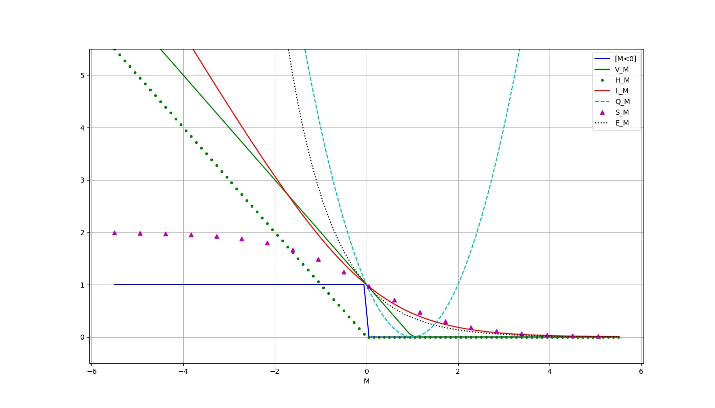
Continuous Approximations of the Threshold Loss Function $\mathcal{L}(M)$
$[M<0]$ — threshold loss function (it is not continuous!)
$V(M) = (1 − M)_+$ — piecewise linear (Support Vector Machine)
$H(M) = (−M)_+$ — piecewise linear (Hebb's rule)
$L(M)=\log_2(1 + \exp(-M))$ — logarithmic (Logistic Regression)
$Q(M)=(1 − M)^2$ — quadratic
$S(M)=2(1+\exp(M))^{-1}$ — sigmoidal
$E(M)= \exp(-M)$ — exponential (let's remember for future AdaBoost)
Linear Classifier — Mathematical Model of a Neuron
Linear model of the McCulloch-Pitts neuron, 1943:
$a(x, w) = f(\left< w, x\right>) = f\left(\sum\limits_{j=1}^n w_j x_j - w_0 \right)$
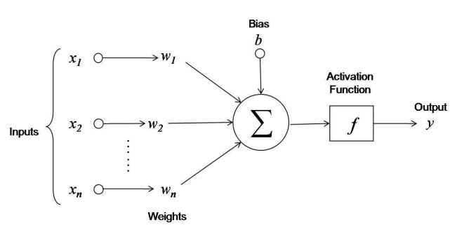
- $f(z)$ — activation function (for example, $\mathrm{sign}$)
- $w_j$ — weight coefficients of synaptic connections
- $w_0 = b$ — activation threshold or bias
- $w, x \in \mathbb{R}^{n+1}$ — if you introduce a constant feature $x_0 \equiv -1$
Gradient Method of Numerical Minimization
Minimization of empirical risk (regression, classification):
$Q(w) = \frac{1}{\ell} \sum\limits_{i=1}^\ell \mathcal{L}_i(w) \to \min\limits_w$Numerical minimization by the gradient descent method:
$w^{(0)} = $ initial approximation
$w^{(t+1)} = w^{(t)} - h \nabla_w Q(w^{(t)})$
where $\nabla_w Q(w) = \left(\frac{\partial Q(w)}{\partial w_j} \right)^n_{j=0}$
$w^{(t+1)} = w^{(t)} - \frac{h}{l} \sum\limits_{i=1}^\ell \nabla_w \mathcal{L}_i(w^{(t)})$
where $h$ is the gradient step, also known as the learning rate
Idea of Speeding up Convergence: take $(x_i, y_i)$ one by one and immediately update the weight vector — stochastic gradient descent.
Visualization of the Gradient Method
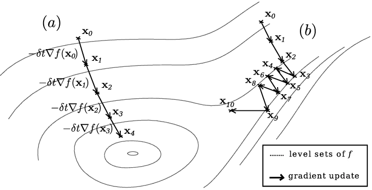
Two possible trajectories of gradient descent:
(a): the target function has "good behavior", which allows the point
to smoothly move to the optimum by the gradient
(b): the gradient begins to oscillate as it falls into a narrow valley,
thus converging more slowly
Stochastic Gradient Descent
Input: sample $X^\ell$, learning rate $h$, decay rate $\lambda$
Output: weight vector $w$
- Initialize weights $w_j,\ j = 0, \dots, n$
- Initialize the estimate of the functional: $\overline{Q} = \frac1\ell \sum\limits_{i=1}^\ell \mathcal{L}_i(w)$
- Repeat:
- Select object $x_i$ from $X^\ell$ randomly
- Compute the loss: $\varepsilon_i = \mathcal{L}_i(w)$
- Make a gradient step: $w = w - h \nabla_w \mathcal{L}_i(w)$
- Assess the functional: $\overline{Q} = \lambda \varepsilon_i + (1 - \lambda) \overline{Q}$
Until the value $\overline{Q}$ and/or weights $w$ converge
Robbins, H., Monro S. A stochastic approximation method // Annals of Mathematical Statistics, 1951, 22 (3), p. 400—407.
Recursive Estimate of Error Functional
Problem: Calculating the $Q$ estimate over the entire selection $x_1, \dots, x_\ell$ is much slower than the gradient step for a single object $x_i$
Solution: Use an approximate recursive formula. Arithmetic Mean:
$\overline{Q}_m = \frac1m \varepsilon_m + \frac1m \varepsilon_{m-1} + \frac1m \varepsilon_{m-2} + \dots$
$\overline{Q}_m = {\color{orange}\frac1m} \varepsilon_m + {\color{orange}\left(1 - \frac1m\right)} \overline{Q}_{m-1}$
Exponential Moving Average:
$\overline{Q}_m = \lambda \varepsilon_m + \left(1 - \lambda\right)\lambda\varepsilon_{m-1} + \left(1 - \lambda\right)^2\lambda\varepsilon_{m-2} + \dots$
$\overline{Q}_m = {\color{orange}\lambda} \varepsilon_m + {\color{orange}\left(1 - \lambda\right)} \overline{Q}_{m-1}$
The parameter $\lambda$ is the rate of forgetting the history of the series.
SAG Algorithm (Stochastic Average Gradient)
Input: sample $X^\ell$, learning rate $h$, decay rate $\lambda$. Output: weight vector $w$
- Initialize weights $w_j,\ j = 0, \dots, n$
- Initialize gradients: $G_i = \nabla \mathcal{L}_i(w), i = 1, \dots, \ell$
- Initialize the estimate of the functional: $\overline{Q} = \frac1\ell \sum\limits_{i=1}^\ell \mathcal{L}_i(w)$
- Repeat
- Select object $x_i$ from $X^\ell$ randomly
- Compute the loss: $\varepsilon_i = \mathcal{L}_i(w)$
- Compute the gradient: $G_i = \nabla \mathcal{L}_i(w)$
- Make a gradient step: $w := w - h {\color{orange} \frac1\ell \sum_{i=1}^\ell G_i}$
- Estimate the functional: $\overline{Q} = \lambda \varepsilon_i + (1 - \lambda) \overline{Q}$
Until the value of $\overline{Q}$ and/or weights $w$ converge
Schmidt M., Le Roux N., Bach F. Minimizing finite sums with the stochastic average gradient // arXiv.org, 2013.
A few tasks to solve (10-15 min)
Weight Initialization Variants
- $w_j = 0$ for all $j = 0, \dots, n$
- Small random values: $$w_j = \text{random}\left(- \frac{1}{2n}, \frac{1}{2n}\right)$$
- $w_j = \frac{\left< y, f_j \right>}{\left< f_j, f_j \right>}$, where $f_j = (f_j(x_i))_{i=1}^\ell$ — vector of feature values
- The loss function is quadratic, and
- The features are uncorrelated: $\left< f_j, f_k \right> = 0, j \neq k$
- Training on a small random sub-sample of objects
- Multi-start: multiple starts from different random initial approximations and choosing the best solution
This estimate of $w$ is optimal if
Variants of Training Object Order
- Shuffling of objects: alternately take objects from different classes
- More frequently take objects with larger errors: the smaller margin $M_i$, the higher the probability to take the object
- More frequently take objects with lower confidence: the smaller $|M_i|$, the higher the probability to take the object
- Do not take "good" objects at all, for those $M_i > \mu_+$ (this can slightly speed up convergence)
- Do not take outlier objects at all, for those $M_i < \mu_-$ (this can potentially improve classification quality)
You will have to adjust the parameters $\mu_+, \mu_-$
Variants of Gradient Step Selection
- Convergence is guaranteed (for convex functions) when
- The method of fastest gradient descent:
- Test random steps for "knocking out" the iterative process from local minima
- The Levenberg-Marquardt method (second order)
$$h_t \to 0, \sum\limits_{t=1}^{\infty} h_t = \infty, \sum\limits_{t=1}^{\infty} h_t^2 < \infty,$$
in particular, you can set $h_t = 1/t$
$$\mathcal{L}_i(w - h\nabla \mathcal{L}_i(w)) \to \min\limits_h$$
allows you to find an adaptive step $h^*$. For a quadratic loss function, $h^* = \|x_i\|^{-2}$
Overfitting Problem
Possible reasons for overfitting:
- Too few objects and too many features
- Linear dependence (multicollinearity) of features:
- Suppose a classifier has been built: $a(x, w) = \mathrm{sign} \left< w, x\right>$
- Multicollinearity: $\exist u \in \mathbb{R}^{n+1}: \forall x_i \in X^\ell \left< u, x_i\right> = 0$
- Non-uniqueness of the solution: $\forall \gamma \in \mathbb{R}\ a(x, w) = \mathrm{sign} \left< w + \gamma u, x\right>$
Manifestations of overfitting:
- Too large weights $|w_j|$ of different signs
- Instability of the discriminant function $\left< w, x\right>$
- $Q(\text{train } X^\ell) \lt\lt Q(\text{test } X^k)$
Main way to reduce overfitting:
Regularization (weight decay)
Regularization (weight decay)
Penalty for increasing the norm of the weight vector:
$\mathcal{\tilde L}_i(w) = \mathcal{L}_i(w) + \frac{\tau}{2} \|w\|^2 = \mathcal{L}_i(w) + \frac{\tau}{2}\sum\limits_{j=1}^n w_j^2 \to \min\limits_w$
Gradient: $\nabla \mathcal{\tilde L}_i(w) = \mathcal{\tilde L}_i(w) + \tau w$
Modification of the gradient step:
$w = w{\color{orange}(1 - h\tau)} - h \nabla \mathcal{L}_i(w)$
Methods for selecting the regularization coefficient $\tau$:
- sliding control
- stochastic adaptation
- two-level Bayesian inference
SG: advantages and disadvantages
Advantages:
- easy to implement
- easy to generalize to any $g(x, w), \mathcal{L}(a, y)$
- easy to add regularization
- possible dynamic (streaming) learning
- on super-large samples, you can get a decent solution, even without processing all $x_i, y_i$
- suitable for tasks with large data
Disadvantages:
- selection of a complex of heuristics is an art (do not forget about overfitting, getting stuck, divergence)
Binary Logistic Regression
-
Linear classification model for two classes \(Y = \{-1, 1\}\):
\(a(x) = \mathrm{sign} \left< w, x\right>\), \(x, w ∈ \mathbb{R}^n\), margin \(M = \left< w, x\right>y\) - Logarithmic loss function: $$\mathcal{L}(M) = \log(1 + e^{-M})$$
- Conditional probability model: $$ P(y|x, w) = \sigma(M) = \frac{1}{1 + e^{-M}},$$ where \(\sigma(M)\) is the sigmoid function, important property: \(\sigma(M) + \sigma(-M) = 1\)
- Regularized logistic regression learning problem (minimization of approximated empirical risk): $$Q(w) = \sum\limits_{i=1}^\ell \log(1 + \exp(-\left< w, x_i\right>y_i)) + \frac{\tau}{2}\|w\|^2_2 \to \min\limits_w $$
Multiclass Logistic Regression
Linear classifier with an arbitrary number of classes \(|Ү|\):
\(a(x) = \arg\max\limits_{y \in Y} < w_y, x>\), \(x, w_y \in \mathbb{R}^n\)The probability that the object \(x\) belongs to the class \(y\):
\(P(y|x,w) = \frac{\exp< w_y, x>}{\sum\limits_{z \in Y} \exp< w_z, x>} = \underset{y \in Y}{\mathrm{softmax}} < w_y, x>\)The \(\mathrm{softmax}: \mathbb{R}^Y \to \mathbb{R}^Y\) function converts any vector into a normalized vector of a discrete distribution.
Maximization of a likelihood (log-loss) with regularization is the same as minimization of approximated empirical risk:
\( L(w) = \sum\limits_{i=1}^\ell \log P(y_i|w, x_i) - \frac{\tau}{2} \sum\limits_{y \in Y} \|w_y\|^2 \to \max\limits_w \)Summary
- The Stochastic Gradient (SG, SAG) method is suitable for any models and loss functions
- Well suited for large data learning
- Approximation of the threshold loss function $\mathcal{L}(M)$ allows the use of gradient optimization
- Functions $\mathcal{L}(M)$, penalizing for the approximation to the class boundary, increase the gap between classes, thereby improving classification reliability
- Regularization solves the multicollinearity problem and also reduces overfitting
- Likelihood maximization and minimization of the empirical risk are different views on the same optimization problem
Principle of maximum likelihood
Let $X \times Y$ be a probability space, and the model (i.e., its parameters $w$) is also generated by some probability distribution.
Bayes' theorem:
$P(A|B) = \frac{P(B|A)P(A)}{P(B)}$
$A \equiv w$, $B \equiv Y, X\ \Rightarrow$
$P(w|Y, X) = \frac{P(Y, X|w)P(w)}{P(Y, X)} = \frac{P(Y | X, w)P(X|w)P(w)}{P(Y | X)P(X)}$
$\boxed{P(w|Y,\ X) = \frac{P(Y|w, X)P(w)}{P(Y | X)}}$
Here: $P(w|Y, X)$ — posterior distribution of parameters
$P(Y|X, w)$ — likelihood, $P(w)$ — prior distribution of parameters
Connection of likelihood and approximation of empirical risk
Maximum likelihood
$L(w) = \sum\limits_{i=1}^\ell {\color{orange}\log P(y_i|w, x_i)} \to \max\limits_w$
Minimization of the approximated empirical risk
$Q(w) = \sum\limits_{i=1}^\ell {\color{orange}\mathcal{L}(y_i, x_i, w)} \to \min\limits_w$
These two principles are equivalent if we set
$ -\log P(y_i|w, x_i) = \mathcal{L}(y_i, x_i, w)$
Model $P(y|x,w) \equiv $ Model $g(x,w)$ and $\mathcal{L}(M)$
Probabilistic interpretation of regularization
\(P(y|x, w)\) — probabilistic data model
\(P(w; \gamma)\) — prior distribution of model parameters, \(\gamma\) — vector of hyperparameters;
Joint likelihood of data and model
\[P(X^\ell, w) = P(X^\ell | w)P(w;\gamma)\]Maximum a Posteriori Probability (MAP) principle:
\[ L(w) = \log P(X^\ell, w) = \sum\limits_{i=1}^\ell \log P(y_i|w, x_i) + \underbrace{\color{orange}{\log P(w; \gamma)}}_{\text{regularizer}} \to \max\limits_w \]How else can the logarithm help?
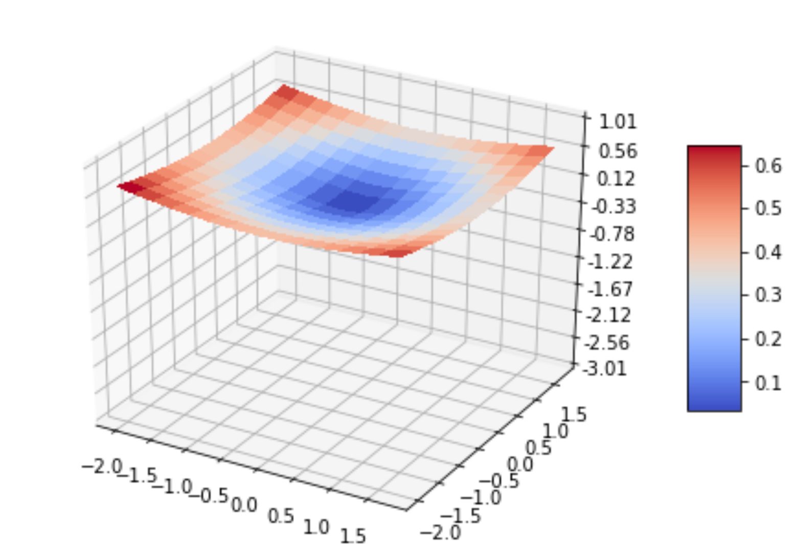
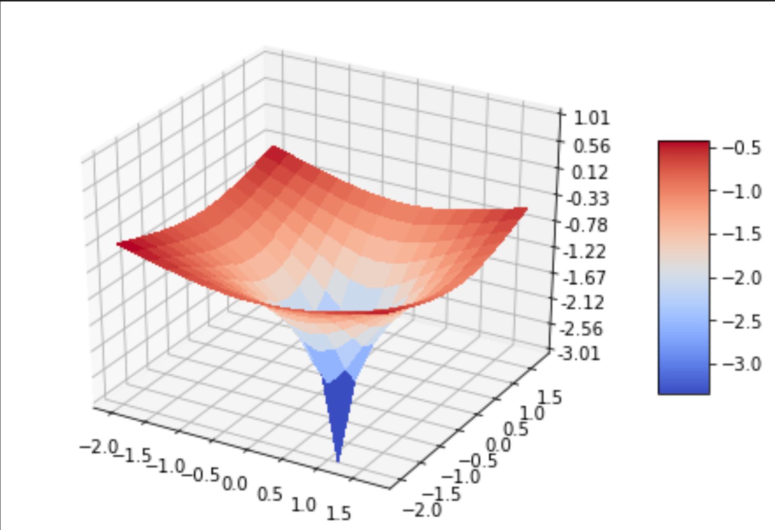
Examples: Gaussian and Laplace priors
Let the weights \(w_j\) be independent, \(\mathbb{E}w_j = 0\), \(\mathbb{D}w_j = С\)
Gaussian distribution and quadratic (\(L_2\)) regularizer:
$$P(w; С) = \frac{1}{(2\pi C)^{n/2}} \exp \left(-\frac{{\|w\|^2_2}}{2C}\right)$$ $${\|w\|^2_2 = \sum\limits_{j=1}^n w_j^2}$$ $$-\log P(w; С) = \frac{1}{2C}\|w\|^2_2 + const$$Laplace distribution and absolute (\(L_1\)) regularizer:
$$P(w; С) = \frac{1}{(2C)^{n}} \exp \left(-\frac{{\|w\|_1}}{C}\right)$$ $${\|w\|_1 = \sum\limits_{j=1}^n |w_j|}$$ $$-\log P(w; С) = \frac{1}{C}\|w\|_1 + const$$\(C\) — hyperparameter, \(\tau = \frac{1}{C}\) — regularization coefficient